Intro to TensorFlow for Deep Learning by Udacity
Introduction
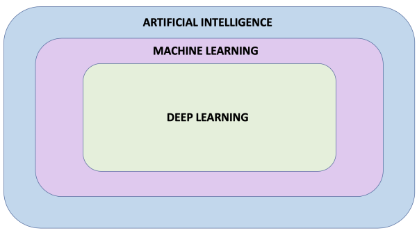
When studying Machine Learning you will come across many different terms such as artificial intelligence, machine learning, neural network, and deep learning. But what do these terms actually mean and how do they relate to each other?
Below we give a brief description of these terms:
- Artificial Intelligence: A field of computer science that aims to make computers achieve human-style intelligence. There are many approaches to reaching this goal, including machine learning and deep learning.
- Machine Learning: A set of related techniques in which computers are trained to perform a particular task rather than by explicitly programming them.
- Neural Network: A construct in Machine Learning inspired by the network of neurons (nerve cells) in the biological brain. Neural networks are a fundamental part of deep learning, and will be covered in this course.
- Deep Learning: A subfield of machine learning that uses multi-layered neural networks. Often, “machine learning” and “deep learning” are used interchangeably.

Machine learning and deep learning also have many subfields, branches, and special techniques. A notable example of this diversity is the separation of Supervised Learning and Unsupervised Learning.
To over simplify — in supervised learning you know what you want to teach the computer, while unsupervised learning is about letting the computer figure out what can be learned. Supervised learning is the most common type of machine learning, and will be the focus of this course.
What is Machine Learning
There are many types of neural network architectures. However, no matter what architecture you choose, the math it contains (what calculations are being performed, and in what order) is not modified during training. Instead, it is the internal variables (“weights” and “biases”) which are updated during training.
For example, in the Celsius to Fahrenheit conversion problem, the model starts by multiplying the input by some number (the weight) and adding another number (the bias). Training the model involves finding the right values for these variables, not changing from multiplication and addition to some other operation.
The Basics: Training your first model
To keep this page from being massive, all codes / projects will be on their own page. Therefore, visit Intro to TensorFlow for Machine Learning by Udacity - Training your first model.
The Training Process
The training process (happening in model.fit(…)) is really about tuning the internal variables of the networks to the best possible values, so that they can map the input to the output. This is achieved through an optimization process called Gradient Descent, which uses Numeric Analysis to find the best possible values to the internal variables of the model.
To do machine learning, you don't really need to understand these details. But for the curious: gradient descent iteratively adjusts parameters, nudging them in the correct direction a bit at a time until they reach the best values. In this case “best values” means that nudging them any more would make the model perform worse. The function that measures how good or bad the model is during each iteration is called the “loss function”, and the goal of each nudge is to “minimize the loss function.”
The training process starts with a forward pass, where the input data is fed to the neural network. Then the model applies its internal math on the input and internal variables to predict an answer.
In our example, the input was the degrees in Celsius, and the model predicted the corresponding degrees in Fahrenheit.
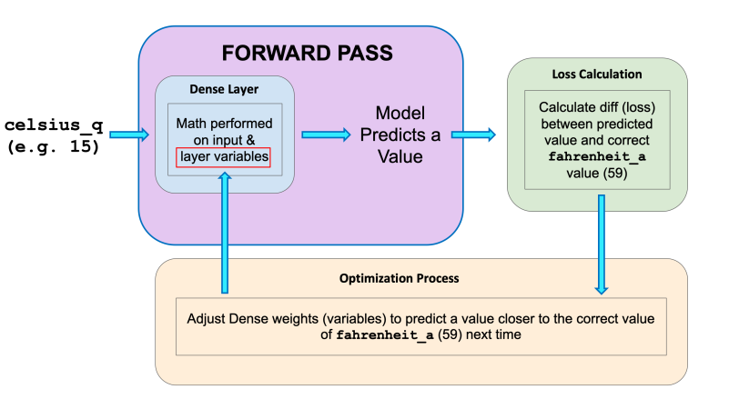
Once a value is predicted, the difference between that predicted value and the correct value is calculated. This difference is called the loss, and it's a measure of how well the model performed the mapping task. The value of the loss is calculated using a loss function, which we specified with the loss parameter when calling model.compile().
After the loss is calculated, the internal variables (weights and biases) of all the layers of the neural network are adjusted, so as to minimize this loss — that is, to make the output value closer to the correct value.
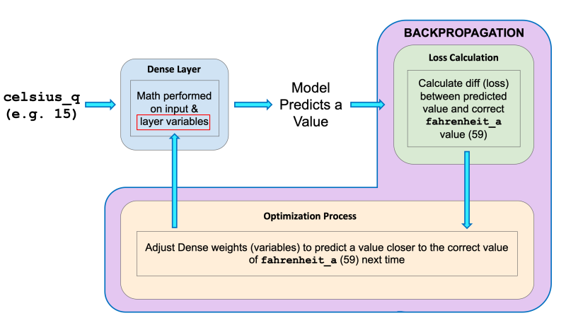
This optimization process is called Gradient Descent. The specific algorithm used to calculate the new value of each internal variable is specified by the optimizer parameter when calling model.compile(…). In this example we used the Adam optimizer.
It is not required for this course, but if you're interested in learning more details about how the training process works, you can look at the lesson on reducing loss in Google’s machine learning crash course.
By now you should know what the following terms are:
- Feature: The input(s) to our model
- Examples: An input/output pair used for training
- Labels: The output of the model
- Layer: A collection of nodes connected together within a neural network.
- Model: The representation of your neural network
- Dense and Fully Connected (FC): Each node in one layer is connected to each node in the previous layer.
- Weights and biases: The internal variables of model
- Loss: The discrepancy between the desired output and the actual output
- MSE: Mean squared error, a type of loss function that counts a small number of large discrepancies as worse than a large number of small ones.
- Gradient Descent: An algorithm that changes the internal variables a bit at a time to gradually reduce the loss function.
- Optimizer: A specific implementation of the gradient descent algorithm.
- Learning rate: The “step size” for loss improvement during gradient descent.
- Batch: The set of examples used during training of the neural network
- Epoch: A full pass over the entire training dataset
- Forward pass: The computation of output values from input
- Backward pass (backpropagation): The calculation of internal variable adjustments according to the optimizer algorithm, starting from the output layer and working back through each layer to the input.
The Rectified Linear Unit (ReLU)
ReLU stands for Rectified Linear Unit and it is a mathematical function that looks like this:
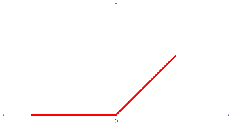
As we can see, the ReLU function gives an output of 0 if the input is negative or zero, and if input is positive, then the output will be equal to the input.
ReLU gives the network the ability to solve nonlinear problems.
Converting Celsius to Fahrenheit is a linear problem because f = 1.8*c + 32 is the same form as the equation for a line, y = m*x + b. But most problems we want to solve are nonlinear. In these cases, adding ReLU to our Dense layers can help solve the problem.
ReLU is a type of activation function. There several of these functions (ReLU, Sigmoid, tanh, ELU), but ReLU is used most commonly and serves as a good default. To build and use models that include ReLU, you don’t have to understand its internals. But, if you want to know more, see this article on ReLU in Deep Learning.
Let’s review some of the new terms that were introduced in this lesson:
- Flattening: The process of converting a 2d image into 1d vector
- ReLU: An activation function that allows a model to solve nonlinear problems
- Softmax: A function that provides probabilities for each possible output class
- Classification: A machine learning model used for distinguishing among two or more output categories
Training and Testing
TensorFlow Datasets provides a collection of datasets ready to use with TensorFlow.
Datasets are typically split into different subsets to be used at various stages of training and evaluation of the neural network. In this section we talked about:
- Training Set: The data used for training the neural network.
- Test set: The data used for testing the final performance of our neural network.
The test dataset was used to try the network on data it has never seen before. This enables us to see how the model generalizes beyond what it has seen during training, and that it has not simply memorized the training examples.
In the same way, it is common to use what is called a Validation dataset. This dataset is not used for training. Instead, it it used to test the model during training. This is done after some set number of training steps, and gives us an indication of how the training is progressing. For example, if the loss is being reduced during training, but accuracy deteriorates on the validation set, that is an indication that the model is memorizing the test set.
The validation set is used again when training is complete to measure the final accuracy of the model.
You can read more about all this in the Training and Test Sets lesson of Google’s Machine Learning Crash Course.
Classifying Images of Clothing
To keep this page from being massive, all codes / projects will be on their own page. Therefore, visit Intro to TensorFlow for Machine Learning by Udacity - Classifying Images of Clothing.
Summary of Classifying Images of Clothing
We trained a neural network to classify images of articles of clothing. To do this we used the Fashion MNIST dataset, which contains 70,000 greyscale images of articles of clothing. We used 60,000 of them to train our network and 10,000 of them to test its performance. In order to feed these images into our neural network we had to flatten the 28 × 28 images into 1d vectors with 784 elements. Our network consisted of a fully connected layer with 128 units (neurons) and an output layer with 10 units, corresponding to the 10 output labels. These 10 outputs represent probabilities for each class. The softmax activation function calculated the probability distribution.
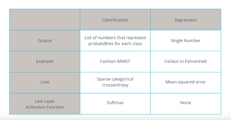
We also learned about the differences between regression and classification problems.
- Regression: A model that outputs a single value. For example, an estimate of a house’s value.
- Classification: A model that outputs a probability distribution across several categories. For example, in Fashion MNIST, the output was 10 probabilities, one for each of the different types of clothing. Remember, we use Softmax as the activation function in our last Dense layer to create this probability distribution.
You can follow this video and accompanying Colab notebook, which covers regression vs classification. It also describes another regression model that predicts the fuel efficiency for different types of cars.
Convolutions and Max Pooling
A convolution is the process of applying a filter (“kernel”) to an image. Max pooling is the process of reducing the size of the image through downsampling.
As you will see in the following Colab notebook, convolutional layers can be added to the neural network model using the Conv2D layer type in Keras. This layer is similar to the Dense layer, and has weights and biases that need to be tuned to the right values. The Conv2D layer also has kernels (filters) whose values need to be tuned as well. So, in a Conv2D layer the values inside the filter matrix are the variables that get tuned in order to produce the right output.
Here are some of terms that were introduced in this lesson:
- CNNs: Convolutional neural network. That is, a network which has at least one convolutional layer. A typical CNN also includes other types of layers, such as pooling layers and dense layers.
- Convolution: The process of applying a kernel (filter) to an image
- Kernel / filter: A matrix which is smaller than the input, used to transform the input into chunks
- Padding: Adding pixels of some value, usually 0, around the input image
- Pooling The process of reducing the size of an image through downsampling.There are several types of pooling layers. For example, average pooling converts many values into a single value by taking the average. However, maxpooling is the most common.
- Maxpooling: A pooling process in which many values are converted into a single value by taking the maximum value from among them.
- Stride: the number of pixels to slide the kernel (filter) across the image.
- Downsampling: The act of reducing the size of an image
If you want to learn / understand more, take a read of A more detailed guide to Convolutional Neural Networks - The ELI5 Way