This is an old revision of the document!
Introduction to TensorFlow for Artificial Intelligence, Machine Learning, and Deep Learning
Week 1:
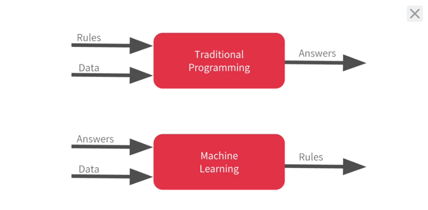
Traditional Programming vs Machine Learning
Hello World of Neural Networks

# One Neuron Neural Network
# Dense = Define a Layer of connected Neurons
# Only 1 Layer, Only 1 Unit, so a Single (1) Neuron

model = keras.Sequential([keras.layers.Dense(units=1, input_shape=[1])])
model.compile(optimizer='sgd', loss='mean_squared_error')

xs = np.array([-1.0, 0.0, 1.0, 2.0, 3.0, 4.0], dtype=float)
ys = np.array([-3.0, -1.0, 1.0, 3.0, 5.0, 7.0], dtype=float)

model.fit(xs, ys, epochs=500)
You've probably seen that for machine learning, you need to know and use a lot of math, calculus probability and the like.
It's really good to understand that as you want to optimize your models but the nice thing for now about TensorFlow and keras is that a lot of that math is implemented for you in functions.
There are two function roles that you should be aware of though and these are loss functions and optimizers.
This code defines them. I like to think about it this way.
The neural network has no idea of the relationship between X and Y, so it makes a guess.
Say it guesses Y equals 10X minus 10. It will then use the data that it knows about, that's the set of Xs and Ys that we've already seen to measure how good or how bad its guess was.
The loss function measures this and then gives the data to the optimizer which figures out the next guess. So the optimizer thinks about how good or how badly the guess was done using the data from the loss function.
Then the logic is that each guess should be better than the one before. As the guesses get better and better, an accuracy approaches 100 percent, the term convergence is used.
In this case, the loss is mean squared error and the optimizer is SGD which stands for stochastic gradient descent.
Our next step is to represent the known data.
These are the Xs and the Ys that you saw earlier. The np.array is using a Python library called numpy that makes data representation particularly enlists much easier.
So here you can see we have one list for the Xs and another one for the Ys. The training takes place in the fit command. Here we're asking the model to figure out how to fit the X values to the Y values.
The epochs equals 500 value means that it will go through the training loop 500 times. This training loop is what we described earlier. Make a guess, measure how good or how bad the guesses with the loss function, then use the optimizer and the data to make another guess and repeat this.
When the model has finished training, it will then give you back values using the predict method.
The Software
Like every first app you should start with something super simple that shows the overall scaffolding for how your code works.
In the case of creating neural networks, the sample I like to use is one where it learns the relationship between two numbers. So, for example, if you were writing code for a function like this, you already know the 'rules' —
''float hw_function(float x){
    float y = (2 * x) - 1;
    return y;
}''
So how would you train a neural network to do the equivalent task? Using data! By feeding it with a set of Xs, and a set of Ys, it should be able to figure out the relationship between them.
This is obviously a very different paradigm than what you might be used to, so let's step through it piece by piece.
Imports
Let's start with our imports. Here we are importing TensorFlow and calling it tf for ease of use.
We then import a library called numpy, which helps us to represent our data as lists easily and quickly.
The framework for defining a neural network as a set of Sequential layers is called keras, so we import that too.
In [0]:
import tensorflow as tf
import numpy as np
from tensorflow import keras
Define and Compile the Neural Network
Next we will create the simplest possible neural network. It has 1 layer, and that layer has 1 neuron, and the input shape to it is just 1 value.
In [0]:
model = tf.keras.Sequential([keras.layers.Dense(units=1, input_shape=[1])])
Now we compile our Neural Network. When we do so, we have to specify 2 functions, a loss and an optimizer.
If you've seen lots of math for machine learning, here's where it's usually used, but in this case it's nicely encapsulated in functions for you. But what happens here — let's explain…
We know that in our function, the relationship between the numbers is y=2x-1.
When the computer is trying to 'learn' that, it makes a guess…maybe y=10x+10. The LOSS function measures the guessed answers against the known correct answers and measures how well or how badly it did.
It then uses the OPTIMIZER function to make another guess. Based on how the loss function went, it will try to minimize the loss. At that point maybe it will come up with somehting like y=5x+5, which, while still pretty bad, is closer to the correct result (i.e. the loss is lower)
It will repeat this for the number of EPOCHS which you will see shortly. But first, here's how we tell it to use 'MEAN SQUARED ERROR' for the loss and 'STOCHASTIC GRADIENT DESCENT' for the optimizer. You don't need to understand the math for these yet, but you can see that they work! :)
Over time you will learn the different and appropriate loss and optimizer functions for different scenarios.
In [0]:
model.compile(optimizer='sgd', loss='mean_squared_error')
Providing the Data
Next up we'll feed in some data. In this case we are taking 6 xs and 6ys. You can see that the relationship between these is that y=2x-1, so where x = -1, y=-3 etc. etc.
A python library called 'Numpy' provides lots of array type data structures that are a defacto standard way of doing it. We declare that we want to use these by specifying the values as an np.array[]
In [0]:
xs = np.array([-1.0,  0.0, 1.0, 2.0, 3.0, 4.0], dtype=float)
ys = np.array([-3.0, -1.0, 1.0, 3.0, 5.0, 7.0], dtype=float)
Training the Neural Network
The process of training the neural network, where it 'learns' the relationship between the Xs and Ys is in the model.fit call. This is where it will go through the loop we spoke about above, making a guess, measuring how good or bad it is (aka the loss), using the opimizer to make another guess etc. It will do it for the number of epochs you specify. When you run this code, you'll see the loss on the right hand side.
In [0]:
model.fit(xs, ys, epochs=500)
Ok, now you have a model that has been trained to learn the relationship between X and Y. You can use the model.predict method to have it figure out the Y for a previously unknown X. So, for example, if X = 10, what do you think Y will be? Take a guess before you run this code:
In [0]:
print(model.predict([10.0]))
You might have thought 19, right? But it ended up being a little under. Why do you think that is?
Remember that neural networks deal with probabilities, so given the data that we fed the NN with, it calculated that there is a very high probability that the relationship between X and Y is Y=2X-1, but with only 6 data points we can't know for sure. As a result, the result for 10 is very close to 19, but not necessarily 19.
As you work with neural networks, you'll see this pattern recurring. You will almost always deal with probabilities, not certainties, and will do a little bit of coding to figure out what the result is based on the probabilities, particularly when it comes to classification.